farblog

I recently refreshed a VM running Debian testing (Forky/Debian 14) and suddenly found that middle-click paste had stopped working… but only in Chrome?!

It turns out that it wasn’t actually only Chrome that was affected, and since this is likely something that I’ll run into again, I’m documenting it here for the next time I need it.

First, what am I talking about? X11 has the concept of both a modern clipboard (cut/copy/paste) and a separate “primary selection”¹ that’s updated whenever the user selects some text. Wayland (which I’m using) supports essentially the same idea.

This effectively gives you two separate clipboards, with one of them more ephemeral than the other. Middle-clicking with the mouse will usually paste from the primary selection, giving you both a ‘regular’ clipboard and a fast way to copy text from one place to another: just select it and middle-click to paste.

And this is the feature that had suddenly stopped working, but apparently only in Chrome; my terminal (foot) was working fine. Obviously, I initially assumed that Chrome was at fault, and it kind of was, but not in the way I expected.

I’ll spare you the trawling through /var/log/apt/history.log, and just explain what happened.

GNOME has for a while offered a setting to control whether middle-click paste is enabled, and Chrome, being approximately a GTK application on Linux, respects that setting.

Now, I’m not using GNOME (I use sway, the Wayland drop-in replacement for X11’s i3 window manager), but GTK applications will still read those GTK settings, even if I don’t have a convenient way to change them.

However, GNOME 50 decided to disable primary paste by default on the basis that it was confusing for new users, so the system default for this setting became false from gsettings-desktop-schemas version 50.0-1.

This affects all GTK applications, not just Chrome. However, at the time I wasn’t running any other GTK applications, so everything else continued to work just fine. (For example, foot is a non-GTK Wayland application, so it just uses Wayland’s native primary selection protocol, and doesn’t look at the GTK setting.)

The default value for this GTK setting comes from a compiled GSettings schema file². In this case the XML source is /usr/share/glib-2.0/schemas/org.gnome.desktop.interface.gschema.xml, which now looks like this:

<key name="gtk-enable-primary-paste" type="b">
  <default>false</default>
  <summary>Enable the primary paste selection</summary>
  <description>
    If true, gtk+ uses the primary paste selection, usually
    triggered by a middle mouse button click.
  </description>
</key>

(Previously, that default was true; that’s the change from gsettings-desktop-schemas.)

Debian does register a script with the user-session-migration package to re-enable this setting on a per-user basis after updating from an older version. That should run via /usr/bin/user-session-migration (which in turn is invoked by a systemd user unit that starts on GUI session startup).

However, firstly, that assumes you realise you need to log out and log in again after upgrading a package, and secondly, that systemd unit doesn’t appear to run at all on my Debian testing VM³.

In any case, that upgrade script also won’t help when I install from scratch (at which point I will definitely have forgotten where this setting is located!).

How to fix this, then? Well, for an upgrade, it is possible that running /usr/bin/user-session-migration might just work, so you could try that first.

Otherwise – and for new installs – changing the setting locally (which is all that script is doing) is the easiest way to revert to the older behaviour. Simply run:

$ gsettings set \
  org.gnome.desktop.interface gtk-enable-primary-paste true

or equivalently (if the gsettings binary from libglib2.0-bin is not installed, which it very well might not be):

$ dconf write \
  /org/gnome/desktop/interface/gtk-enable-primary-paste true

This updates ~/.config/dconf/user, and takes effect immediately (in Chrome, at least).

It’s slightly annoying that a default change in a desktop environment I’m not using was responsible for breaking functionality in a browser I am, but at least now I’ll know where to look the next time I need to understand this.

In a footnote to a previous post, I mentioned that I’d recently done some TCP tuning to increase initcwnd on this website, which runs on Google Compute Engine (GCE from here on out). Configuring this turned out to be surprisingly tricky, so I thought it would be useful to write up how it all fits together and how to do this on GCE.

Note that I’m specifically going to be talking about the Debian 13 (Trixie) cloud images, which configure networking via systemd-networkd managed by Netplan. Netplan isn’t critical here, but if you’re not using systemd-networkd, this post probably won’t be that useful.

First, what was I trying to achieve?

initcwnd is the TCP initial congestion window, and controls how much data a server can transmit at the start of a connection before it needs to wait for an acknowledgement from the client.

Linux 2.6.39+ defaults to an initcwnd of 10 segments¹ (up to 10 × MSS bytes). On GCE, where the default virtual network MTU is 1460 bytes, this allows transmitting almost 14 KiB in a single go. For a webserver, this means that if an HTTP response (including headers) is larger than that, the server must pause partway to wait for the client to send a TCP ACK, and only then continue with the remainder of the response.

Increasing initcwnd to 20 segments is therefore a quick way to reduce latency for small (approximately, 14–28 KiB) responses, since it effectively cuts their transfer time in half. For most webservers, there’s quite a lot that fits in that size range: for example, while this post by itself is comfortably smaller than 14 KiB (assuming compression), my front page (compressed) will typically be just a little larger than that threshold.

The hard limit for the initial TCP window is 65535 bytes, which in practice would be about 44 segments². However, setting initcwnd higher than about 20 is usually not recommended: sending too many packets can overflow intermediate routers’ receive buffers (leading to packet loss – and packet loss during the initial TCP connection can stall the connection for seconds), and can also contribute to bufferbloat, potentially causing latency spikes for other traffic. 20 is a ‘reasonable’ figure that noticeably improves latency without triggering any of those side effects.

Note that this does assume that the ultimate receiver can actually handle this much data: some very old mobile clients and modern IoT clients (and e.g. Windows XP) will advertise a smaller receive window (their initrwnd), which will cap the size of the initial window.

Anyway, that’s why I wanted to configure initcwnd on this webserver (also, because it’s fun). The rest is how to do so.

As is common, on the GCE version of Debian, the internal IPv4 address is set by DHCP. As is slightly less common, DHCP also provides the server with default and gateway routes (per RFC 3442).

In modern versions of systemd, systemd-networkd can be told how to set initcwnd via an InitialCongestionWindow setting in a .network file.

We can see which .network file systemd-networkd is using with networkctl status (which accepts interface names or shell-style wildcards):

$ networkctl status 'en*'
● 2: ens4
                   Link File: /usr/lib/systemd/network/99-default.link
                Network File: /run/systemd/network/10-netplan-all-en.network
                       State: routable (configured)
...

(or networkctl with no arguments will list all the network links that systemd-networkd is aware of.)

Network File: is the important part here: it shows the name of the .network file that we’d need to change.

However, here we have a dynamic file (in /run/) generated by Netplan, so we can’t modify it directly. Fortunately, systemd-networkd also supports the idea of “drop-in files” that can be used to add additional configuration to an existing network; see man systemd.network.

For example, for the network link above, we could put extra configuration into /etc/systemd/network/10-netplan-all-en.network.d/*.conf, where the name of the .d directory has to match the name of the network file.

So here we’d just need to add a [DHCPv4] section with InitialCongestionWindow=20 to achieve what we want to do.

This approach does rely on the Netplan-generated filename staying static, but that should be the case: it seems to use a hardcoded 10-netplan- prefix, plus a string from the /etc/netplan/ configuration, which should be unlikely to change. Of course, if you’re not using Netplan, it’s even easier, since you just edit the .network file directly.

So IPv4 is pretty simple, once we know what file to create (I’ve put a complete example below), but IPv6 is a little more mysterious.

For IPv6, you might expect to be able to add a similar setting under one of the IPv6-related sections, but the specific setting we’re after can only be specified under [Route] and [DHCPv4], at least as of systemd 261³.

We do have a solution, thankfully, but it requires understanding how routing is configured for dynamic IPv6:

The IPv6 address is assigned by stateful DHCPv6, where systemd-networkd runs a client to lease the public /128 address from its allocated subnet. GCE does not use SLAAC for address assignment. However, DHCPv6 only provisions addresses, not routes.

The IPv6 route is assigned by watching for periodic ICMPv6 Router Advertisement broadcasts⁴.

When an RA packet arrives, systemd-networkd processes it and normally installs the default route. RA packets only supply IPv6 routing parameters (and we can’t change what GCE sends anyway), and as noted above, systemd-networkd doesn’t have any obvious place to attach route metrics like initcwnd to the result.

Fortunately, we can switch off the automatic creation of that default route and instead configure a route of our own that will become the default route.

To cut to the chase, we can set initcwnd for both IPv4 and IPv6 by creating a single drop-in file with a name matching the network file shown by networkctl status:

# /etc/systemd/network/10-netplan-all-en.network.d/initcwnd.conf
[DHCPv4]
InitialCongestionWindow=20

[IPv6AcceptRA]
UseGateway=no

[Route]
Destination=::/0
Gateway=_ipv6ra
InitialCongestionWindow=20

Setting UseGateway=no stops systemd-networkd from creating its own default route when receiving the RA; instead, it finds the [Route] that defines Gateway=_ipv6ra, and installs that route using the advertised gateway. Since our route also defines Destination=::/0, it becomes the default route.

While my focus was on initcwnd, you can obviously also use this to set any other per-route settings, such as InitialAdvertisedReceiveWindow (initrwnd). Some other per-route settings can already be set directly in the [IPv6AcceptRA] section, which is probably a better place for them. (If a future version of systemd adds support for the missing settings to [IPv6AcceptRA], the above would become a little simpler.)

sudo networkctl reload reloads the configuration and updates the IPv4 route immediately from the cached DHCP lease. For IPv6, it’ll drop the default route (the one created by UseGateway=yes) and request a new RA by sending out a Router Solicitation packet. That should trigger a new RA, installing the new IPv6 default route within a second. (Alternatively, you can just reboot the VM.)

Once everything’s been updated, we can see the results with ip route:

$ ip -4 route show default
default via 10.154.0.1 dev ens4 proto dhcp src 10.154.15.203 metric 100 initcwnd 20

$ ip -6 route show default
default nhid 886644799 via fe80::4001:aff:fe9b:1 dev ens4 proto ra metric 100 expires 85sec initcwnd 20 pref medium

The two via addresses are the local gateways, and proto dhcp and proto ra show what protocols provided the routes: DHCP for the IPv4 route, and a Router Advertisement broadcast for the IPv6 route. Both now have initcwnd 20, which was what I wanted to achieve.

Well, it took a bit of digging through man pages to figure out what was going on here, but the end result is that I now have a much better understanding of modern networking clients, and of IPv6 – which was really the main reason I wanted to look into this in the first place. Writing it up here should also give me a place to look the next time I want to remember what’s going on.

Oh, and this server is very slightly faster now too.

Here’s the tl;dr (also, spoilers): if you’re using Prometheus’ blackbox exporter to probe a target, you should probably explicitly specify the IP protocol (IPv4 or IPv6) to use for each probe, especially if you have an IPv4-only target.

I have a very small home monitoring setup using Prometheus and various exporters to monitor this website, plus a few other sites and machines that I care about. For HTTP monitoring, I’m using Prometheus’ blackbox exporter to probe a target URL (the front page of this site) every so often.

The probe configuration is a little bit confusing, as the targets (what to monitor, i.e. the target URL) are set in the main Prometheus config, while the probe definition and expectations (how to monitor) are set in the blackbox exporter config, but the latter looks something like this:

modules:
  farblog_https:
    prober: http
    http:
      headers:
        accept-encoding: br
      compression: br
      fail_if_not_ssl: true
      follow_redirects: false
      fail_if_body_not_matches_regexp:
        - "farblog"

This probe succeeds if the site is responding reasonably, and each probe attempt also records various metrics that I can use elsewhere (probe_ssl_earliest_cert_expiry, probe_success, etc).

The automated checks I’m running are pretty basic: verifying that the site is up, that the TLS certificate isn’t about to expire, that kind of thing, but I also have some basic monitoring for probe latency, mostly to detect accidental regressions (or just let me know if something weird is going on).

In the past I’ve used this historical record to test the impact of server changes (for example, I now pre-generate compressed gzip and Brotli representations of most content, which saves a few milliseconds), but as with most things here, it’s just a fun little project to play with.

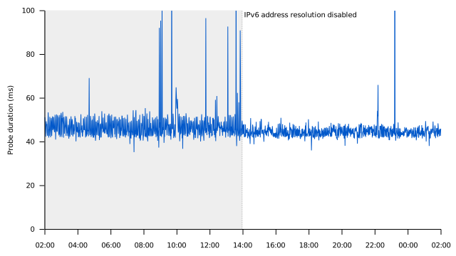
For some time though, I’d been aware that the response times I was seeing were a little spiky, which bothered me: my home internet connection should be fairly stable, and the site itself (which is running nginx on a small GCE node) should be very predictable, and yet my graphs still looked like this:

I’d assumed that this was down to something in my home networking setup that I hadn’t taken account of, but then more recently I noticed that most of the probes to other sites were much more consistent; so what was the difference with this one?

Zooming in to show an hour rather than the whole day (the highlighted part of the graph above) initially didn’t help much, but breaking down the probe duration by the different probe stages (the probe_http_duration_seconds metric) does show something interesting:

This graph is fairly unsurprising: as a static site, most of the time is determined by the number of roundtrips we need to make from the probe origin to the target¹, but the resolve stage is clearly the issue here.

Isolating just resolve makes this even clearer:

This is why my probe latencies were spiky: address resolution usually takes a little over a millisecond, but every so often, it takes about 7 ms instead. What’s going on here?

1–2 ms is about² the time it takes to resolve an address that’s cached by my router, while 7 ms is about³ the time it takes to resolve the target address via my upstream nameservers, so something was clearly making extra queries to my upstream.

My router should definitely be caching the DNS results, and while we absolutely would expect to see a spike when that cached result expires, that should manifest as an extra delay once every 12 hours (the TTL for www.farside.org.uk) – not what we’re seeing here.

One possibility I considered was that my router was prematurely evicting results from its cache, but it’s pretty clear from the graph that “every so often” is actually “every five minutes”, and that’s a big clue: the MINIMUM time for my domain (in the SOA record) is 300 seconds, or five minutes, so this is likely a negative cache result expiring and triggering a query to an upstream nameserver (per RFC 2308). But what non-existent name could it be trying to resolve?

The answer turns out to be IPv6.

At the time I was looking into this, this site only served over IPv4 – GCE didn’t support IPv6 until 2022 or so, and I’d never gone back to turn it on – and so it only had an A record for the IPv4 address, not the AAAA record needed for IPv6.

Somewhat unexpectedly, blackbox exporter’s default behaviour is to resolve both A and AAAA records in parallel, and then only continue once both queries have an answer.⁴

Since in my case there was no AAAA record to resolve, my upstream nameserver would return a NODATA response, and my router would dutifully cache that for the amount of time specified in the SOA record.

The solution is to tell blackbox exporter to resolve only one address family by disabling ip_protocol_fallback, and then to pick a protocol (or use the default of IPv6) using preferred_ip_protocol:

modules:
  farblog_https:
    prober: http
    http:
      # (as before…)

      # Prefer IPv4, and disable protocol fallback so that we only
      # attempt to resolve an address for one address family.
      preferred_ip_protocol: "ip4"
      ip_protocol_fallback: false

This is also what you’ll want to do if you have an IPv4-only client probing a target that does have an IPv6 address, though in that case it’ll be a lot more obvious, as blackbox exporter will resolve both and then fail to connect via IPv6.

With this change, blackbox exporter only issues a single A record query, which will usually be cached locally. The effect was immediately visible:

This was also the explanation as to why only some of my probes were noticeably affected by this problem: the others were probing dual-stack targets, where the IPv4 and IPv6 addresses would both exist, and would typically have comparable TTLs. This still wasn’t ideal, since the probes would be waiting for answers to DNS queries they wouldn’t use, but in practice it didn’t have anywhere near the same effect on the probe duration.

I do think that blackbox exporter’s default behaviour is a little unfortunate here, since it abstracts away too many of the details (and until fairly recently, was mostly undocumented). However, the documentation has now been updated to describe the address selection process, and to recommend that dual-stack targets, at least, should have separate IPv4 and IPv6 probes.

Does any of this matter to my little website? Of course not, but I had fun digging into the problem, and learned a fair amount along the way. And maybe this write-up will be useful to someone else too.

Coda

In related news, this finally prompted me to put in the work to enable IPv6 on this site, which turned out be to pretty trivial to do. So now I have two separate sets of latency metrics to look at!

(The title of this post is derived from RFC 8305, the “Happy Eyeballs” algorithm that helps applications to connect to dual-stack hosts. While a low-level prober isn’t the kind of application that would actually want to use this algorithm, I thought the reference was too good to pass up!)

I’ll freely admit that I don’t need to use a lot of maths¹ in my day job: pretty much the only things I really need to understand are basic statistics and, occasionally, how to run a t-test to see whether an optimisation has actually improved things (though I guess I don’t even need to understand the maths for that one).

But sometimes maths ends up happening anyway, and it can be interesting when that happens. Here’s one such story:

Let’s say that we have some frontend service that we’d like to understand the performance of in a production configuration. Maybe we want to understand its RAM usage under load, or the latency for some given types of requests, that kind of thing.

In our example system, we’ll send requests to a single frontend task, but there’s a wrinkle: that frontend uses a sharded or replicated backend RPC service to service these requests, and the frontend will only connect² to a given backend task when needed. That connection setup will take a little extra time whenever it occurs, which we don’t want to count in our test.

If we keep sending requests, then eventually the frontend task should have connected to all the backend tasks, and we’ll have a steady-state we can start analysing.

The question then is, how long will it take for our system to set up all of these connections and reach that steady-state? Or, more precisely, how many warm-up requests do we need to send before we can start our real measurements?

Let’s say that our frontend has a hundred backend tasks that it can connect to, and that we’ll model the selection of each backend task as uniformly random for each request. Do we need to send a few hundred requests to our frontend before all of those backends are connected, or a few thousand? Or more?

Incidentally, when I did something like this for real, I used a pragmatic solution instead: keep sending requests until the metric I was monitoring looked like it had settled down, then start measuring. But it did make me wonder how we might go about calculating this mathematically.

Back-of-the-envelope maths time: we know that it has to be at least 100 requests, since we can only make at most one connection to a backend task for any given frontend request. We also know that doing it in exactly 100 requests should both be possible and extremely unlikely:

1. The first request we send will definitely trigger a connection to some backend task, since we haven’t made any connections at all yet.
2. The second request will probably make another connection. Since we have 100 backend tasks, the chance is only $1 / 100$ that we pick the same backend as we used for the first request, so in $99 / 100$ cases we’ll connect to a new backend task.
3. The third request will connect to a third backend in $98 / 100$ cases, and so on.

After we’ve sent that 100^th request, the chance that we’ve connected to all 100 backends is therefore:

$$ \eqalign{ &\frac{100}{100} \times \frac{99}{100} \times \frac{98}{100} \times \dots \times \frac{2}{100} \times \frac{1}{100}\cr = &\frac{100!}{100^{100}} } $$

… which is a very small number: about 1 in $10^{42}$.

So if we want to have a high chance of having connected to all of the backend tasks, we’ll definitely need more than 100 requests, but it’s still not very clear how many: in theory, it could take an unbounded number of requests, since we might never pick all 100!

It turns out that this problem has a name: it’s the coupon collector’s problem, based on the idea of collecting all of $n$ different coupons by drawing randomly, one-by-one.

Calculating the expected number of requests we need is fairly straightforward: we can just sum the expected number of requests we need to make each new connection:

1. For the first connection, we always need exactly one request.
2. For the second connection, the probability of making a new request is $99 / 100$, so the expected number of requests we need is $100 / 99$.
3. For the third connection, the expected number of requests is $100 / 98$, and so on.

To make the last connection, we expect that it’ll take $100 / 1$ or 100 requests, which makes sense: we have to pick the one unconnected backend from 100 options (in the same way that on average you’d expect to need to make six die rolls on a regular six-sided die in order to roll some pre-chosen number).

So, as Wikipedia tells us, if we calculate³

$$ \sum_{k=1}^{n} \frac{n}{k} $$

for n=100, we get about 518.74, which is the expected number of requests we’d need to send.

But what does this number actually tell us? If we send 519 requests, does that mean that we’ll probably have connected to all of the backends? Or that we have exactly a 50% chance of having done so? How many requests do we need if we want to have a 95% chance of having connected to all of the backends, say?

What we’ve just calculated is the expected value, and is an average of the number of requests.

In other words, if we were to run this experiment a large number of times, counting the number of requests until we successfully connected to all the backends ($C_1, C_2, C_3, \dots$), then the expected value is simply the average of those counts.

Since some of these counts might be quite large, this expected value isn’t actually that useful for thinking about the number of requests we’re going to need to send. What we really want to know is what the actual distribution looks like.

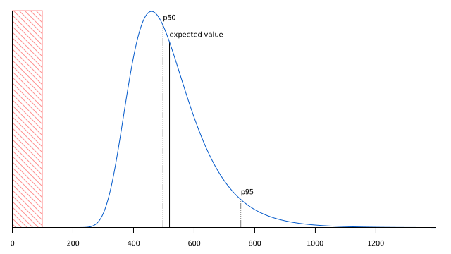
Since randomly picking those last few backends takes quite a few requests, the distribution is heavily skewed to the right. To cut to the chase, it looks like this:

For every point $x$ on the x-axis, the height of the curve shows the probability of collecting 100 coupons – or connecting to all 100 backends, in our example – in exactly $x$ attempts, so for $x = 100$ we have the very small (but non-zero) probability we calculated earlier, while for $x \lt 100$ (the hatched area) the probability is zero, as those values are impossible.

The expected value (518.74) we calculated above is marked, as are the median (497) and 95^th percentile (754). All of these are larger than the mode (460), which is the most-likely number of attempts we’d need.

This graph also has non-zero values everywhere for $x \geq 100$, though it drops off quickly: the probability that we’d take more than 1000 attempts is only 0.4% or so, for example.

Wikipedia goes into the details of how to calculate this distribution exactly, though I don’t feel competent enough to explain it here. One useful nugget, though, is that we can estimate some of the statistics if we map this distribution to what is apparently called a Gumbel distribution:

• The mode for any given $n$ coupons is approximately $n \ln{n}$.
• For any percentile $p$, we can compute $k_p \approx n \ln{n} - n \ln{\left(-\ln{p}\right)}$.

For example, for $n=100$ and $p=0.95$, this gives a mode of 460, which is correct, and a 95^th percentile of 758, which is pretty close to the real value of 754.

In this example, we could be very sure (~99.57%) that if we were to send about a thousand requests, we’ll have connected to all of our backends.

So, the next time you need to work out how many requests it takes to warm up a cache or fill a connection pool, you could use this to work out some magic numbers. But there’s an important caveat for this specific example: all of the above relies on our initial assumption that picking a backend is uniformly random.

In our non-spherical-cow world, load balancers don’t pick backends at random, and instead use a round-robin or similar strategy that would most likely end up actively picking the unconnected backends, significantly reducing the number of requests we actually need to connect to everything.

Maths gives us an interesting worst-case upper bound, but it also suggests why the pragmatic solution was a better idea: sometimes it’s just easier to watch your latency metrics until they flatten out, and let the maths happen in the background.